
GLG410 3-D graphics in Matlab
One of the important tasks we have is the visualization of data that have
been observed at different locations. We often want to compare the values
of certain variables across our observation domain. To do this, we use
contour maps and 3D views of surfaces because often that spatial
distribution of a variable can be thought of as a surface, just like
topography.
Basic ideas of contouring
Middleton talks about the basic rules of contouring in Chapter 8: Spatial
data in his book:
- Contour lines do not cross;
- Contour lines cannot merge with other contour lines;
- Contour lines pass between control points with values higher and
lower than the contour value;
- Contour lines are repeated to indicate a reversal in slope;
- Contour lines must close, or end at the edge of the map.
Contouring can be subjective if done by hand and it almost always has some
influence that comes from the method of contouring if it is done on a
computer. As Middleton points out, there are three separate stages in
contouring, each with its own set of algorithms:
- Griddign: irregularly spaced data must be converted to a set of
oints on a regular grid;
- Location of points: values at gridpoints are not the values
required for contour lines, so points having these values must be found
by interpolation;
- Line drawing: a technique must be chosen for connecting these
points on a contour by a line. In advanced applications, it is
generall required that the line be a smooth curve.
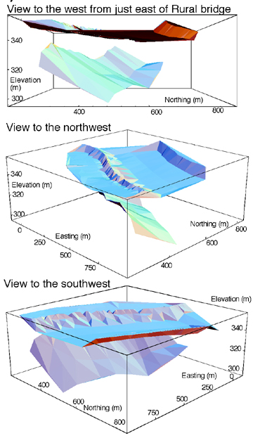
Topography
Topogrpahy is a set of elevation versus location data. We visualize it
commonly by making topographic maps. Here is one for the area of the
Tempe Town Lake:
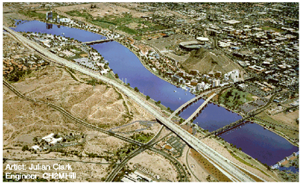
Views of the Tempe Town Lake (TTL) study area and our ongoing
geophysical studies there. A) Design view of TTL illustrating its
situation in the Salt River Channel just north of ASU. B) ASU Field
Geophysics study area with surveyed levee topographic data and also gravity
observation points overlain on pre-levee topographic map of the area. C)
Topography and alluvium-bedrock interface based on gravity model
illustrating the variablility of the alluvium-bedrock interface in the
Pagago Narrows.
THe last figure is obviously not a contour map, but we will talk about 3D
views later this week.
Look at
this page for a study on contouring for one topographic dataset.
Items for Lab
Check out the Electron density
demo.
Look at the contouring and 3D graphics section of the Matlab book.
Pages maintained by
Prof. Ramón Arrowsmith
Last modified November 16, 1999