


Matlab is a program that has been developed for the general solution of mathematical equations, data processing, and data display. MATLAB is an acronym for MATrix LABoratory and it is a highly optimized numerical computation and matrix manipulation package. It is an excellent tool for developing numerical models of problems, performing mathematical operations on large data sets, displaying data in one, two, three, or four dimensions, and solving simultaneous equations. In general, Matlab has been developed as a numerical tool and so best works on real numbers, rather than symbolic operations. However, some versions of Matlab (for example, the Solaris version) are capable of symbolic solutions of equations, symbolic integration and differentiation, and reduction of symbolic equations. The IRIX (Silicon Graphics Incorportated ) version is not capable of many symbolic operations at this time.
In short, if you can write an equation that you think represents a relationship between two or more variables and need to graph your results, Matlab is the tool to use. First, we will go through a short introduction on Matlab concepts, entry formats, graphics, M-files, and functions.
First and foremost, it is important to know how to start Matlab. To start up the program, log into Alai or Darkwing (both machines have about the same version of the software). At the prompt, type ``matlab''. This will start the program. If you are telneting to the machine, graphics will be disabled; however, if you are on the console or are using an XDMCP connection (i.e., eXodus) to one of the machines, you will be able to display graphics. The standard Matlab prompt is ``$>>$'', so once you get this prompt, Matlab is ready to be used.
Matlab can be used like a calculator with standard arithmatic operations on numbers.
>> 1+2

ans =

     3

>> 45-9

ans =

    36

>> 34*9.9

ans =

  336.6000

>> 12/4

ans =

     3
Notice that all un-named operations produce and immediate output in the
form ans = value. The symbol ans is actually a variable which can then be
used in another calculation:
>> 45 *pi/180

ans =

    0.7854

>> sin(ans)

ans =

    0.7071
You can use the power operator (^):
>> 5^3

ans =

   125
It is a good idea to nest things in parentheses in the usual way so that the order of operations is clear:
>> 3 * (sin(4) + sqrt(6)) / 12.5

ans =

    0.4062
If you type in a complex expression and make an error, you can edit the previous expression by pressing the Up arrow on your keyboard to recall the last line. Press the Up Arrow or Down Arrow several times to recall other recent command lines. Use the Left and Right Arrow to move through the command and insert numbers or text or you may also delete something.
Matlab is a vector-based program and works most efficiently if you can pose your problem in the context of vector, matrices, and tensors. In general, all mathematical operations are performed on matrices (a vector is a one column/row matrix, a single number is simply a one element matrix). In order to assign values to a matrix, you need a variable name for the value (which should have some significance to the variable in the problem you are addressing). Here is how to make a variable assignment:
>>myVariable = 6
You will notice that Matlab will echo your output by saying:
myVariable =

     6
If you do not wish to see a confirmation of your assignment, include a semicolon after the operation. This rule holds for all assignments or operations-- if you do not want to see the result of the operation, but simply wish to store it in another variable, use a semicolon:
>> myVariable = 6;
The assignment that you have just made consists of a one element vector. If you wish to assign an entire vector to a variable, enclose the vector's values in brackets. Columns are designated by spaces, while rows are designated by semicolons. For example
>> myVariable = [1 2 3 4 5 6 7 8 9 10]

myVariable =

     1     2     3     4     5     6     7     8     9    10
creates a ten element row vector on which operations can be performed. To create a column vector, instead of spaces, use semicolons:
>> myVariable = [1; 2; 3; 4; 5; 6; 7; 8; 9; 10;]

myVariable =

     1
     2
     3
     4
     5
     6
     7
     8
     9
    10
This creates a ten element column vector with the assigned values for each
of the elements. A row vector is the transpose of a column vector,
therefore, you can use the transpose command to convert from a row vector
to a column vector and vice versa. The transpose command can be called in
a couple of different ways. The first is to use the
transpose() command which will return the transpose of the
vector that you give the command:
>> newVariable = transpose(myVariable)

newVariable =

     1     2     3     4     5     6     7     8     9    10
will return the transpose of myVariable and store the result
in newVariable. Alternately, you could specify that the result of the
transpose could be stored back into myVariable, and thus you
are directly converting myVariable from a column vector to a
row vector or vice versa:
>> myVariable = transpose(myVariable)

myVariable =

     1     2     3     4     5     6     7     8     9    10
The other way to transpose a vector is to use the '
(forward single quote) shorthand:
>> myVariable = myVariable'

myVariable =

     1
     2
     3
     4
     5
     6
     7
     8
     9
    10
Another way that you can make a vector assignment is to assign each element
one after the other by using array notation. In this notation, the
jth element of the vector myVariable is
represented by myVariable(j). Therefore,
you could assign a three element vector with the following commands:
myVariable(1) = 1;
myVariable(2) = 2;
myVariable(3) = 3;
These commands are equivalent to the following command:
>> myVariable = [1 2 3];
The final transition is from vectors to matrices. A vector is a one row or column matrix; therefore, a set of i row vectors of length j forms the i x j matrix (a matrix with i rows and j columns). Matrix assignments can be made as follows:
>> myMatrix = [1 2 3;4 5 6;7 8 9]

myMatrix =

     1     2     3
     4     5     6
     7     8     9
Thus creating the 3 x 3 matrix. To reference some element of the matrix, you can refer to it by its indices:
>> myMatrix(1,2)

ans =

     2

>> myMatrix(2,1)

ans =

     4
to reference the entire first column, you can use a wildcard symbol (the colon):
>> myMatrix(:,1)

ans =

     1
     4
     7
how about the first row?
>> myMatrix(1,:)

ans =

     1     2     3
An alternative way to assign values to a matrix is to use the element array
assignment method. This method is the same as assigning elements in a
vector; however, elements of a matrix are denoted as (i,j)
elements. For example, to set the element in the ith
row and jth column of the matrix
myMatrix to 2, use the
>>myMatrix(i,j) = 2 command at the
Matlab prompt. To set up the matrix myMatrix shown above, you
can issue the following commands:
>> myMatrix(1,1) = 1;
>> myMatrix(1,2) = 2;
>> myMatrix(1,3) = 3;
>> myMatrix(2,1) = 4;
>> myMatrix(2,2) = 5;
>> myMatrix(2,3) = 6;
>> myMatrix(3,1) = 7;
>> myMatrix(3,2) = 8;
>> myMatrix(3,3) = 9;
Those are the basics of variable assignment which is the first thing that you should learn with Matlab. Now that we have assigned variables, we can start to manipulate the variables in order to perform mathematical operations.
A is not the same as
a. Variable names can be up to 32 characters long.
radius_of_curvature and _time are perfectly valid. A space is not
allowed in a variable name (nor most other special UNIX
characters (/,%,&, etc.).
>> pi

ans =

    3.1416

>> inf

ans =

   Inf
If you need to make variables that increment regularly, Matlab has some simple built-in functions to do this. For example, if you need to create a vector that starts at 1 and ends at 100 with a spacing of 1:
incrementVector = [1 2 3 4 5 6 ... 100]
just use the command:
>> x=1:1:100;
Notice that the first number in the assignment is the starting point, the second number is the increment, and the third is the ending point. Both the starting and ending points are inclusive; therefore, the above command creates a 100 element vector.
This command is very useful when setting up a domain for the independent variable(s) in an analysis. In addition, graphics in Matlab are made easier with is feature. Below, we will see how the incremental vector is used in both analysis and graphics.
Once you have created one or more vectors, you can perform mathematical operations on these vectors. Adding and subtracting matrices, vectors, and elements uses the same syntax for each operation and is independent of matrix dimension. For example, if you would like to add vector a to vector b and store the result in vector c, you would type something like the following:
>> a = [1 2 3]

a =

     1     2     3

>> b = [1 2 3]

b =

     1     2     3

>> c = a + b

c =

     2     4     6
The key points are that the two vectors a and b need to be defined already and that the matrix dimensions have to agree:
>> d = [1 2 3 4]

d =

     1     2     3     4

>> e = a + d
??? Error using ==> +
Matrix dimensions must agree.
Likewise, if you would like to subtract vector b from vector
a and store the result in vector c, use the
command:
>> c = b - a

c =

     0     0     0
As with any matrix addition or subtraction, the operation is elementwise,
thus both vectors a and b must be the same
dimensions and the resultant vector c will have the dimensions
of vectors a and b.
As in linear algebra, multiplication of matrices must be more specific due
to the fact that there are two ways to multiply a matrix (i.e. dot product
of two matrices or cross product of two matrices). If you wish to take
the dot product of the matricies a and b
(elementwise multiplication of matrix a and matrix
b[i.e., c(1,1)=a(1,1)*b(1,1) and c(1,2)=a(1,2)*b(1,2),
etc.), and store the result in matrix c use the following
command:
>> c = a.*b

c =

     1     4     9
Notice that when you take the dot product of two matrices, they must have the same dimensions and the resulting matrix will also have those dimensions. You can also do element-by-element division:
>> c = a./b

c =

     1     1     1
Here is an explanation of the action of the dot product on 2 2x2
matrices: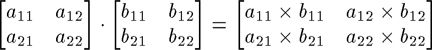
If you need to take the cross product of a two matrices a and
b and store the result in matrix c, use the
following command:
>> c = a * b

c =

    18
When taking the cross product of two matricies, the dimensions of matrix
a must be (i,j) and the dimensions of matrix
b must by (j,i). The resulting matrix
c will have dimensions of (i,j). Here is the cross
product (basically a pair of simultaneous equations):
To raise an element to a power, use the power operator in Matlab,
which is a ^. For example, if you would like to raise a matrix or
vector to a power of 2 (using cross products), type:
>> z = [2 2; 1 2]

z =

     2     2
     1     2

>> c = z^2

c =

     6     8
     4     6
Notice that when you do this, the matrix z must be square. If you would
like to perform a power operation elementwise on a matrix or vector, use
the .^ operator:
>> c = z.^2

c =

     4     4
     1     4
Square roots are easily computed with fractional powers.
If you would like to find the inverse of a matrix (note that z-1
cross product with z = the identity matrix (0s everywhere except 1s on the
diagonal)0, you can use the
inv() command in Matlab. For example, if you would like to
find the inverse of the matrix z and store the result in
matrix c, use the following command:
>> c = inv(z)

c =

    1.0000   -1.0000
   -0.5000    1.0000
These are the basic arithmetic operators that you will use in Matlab. Remember to be careful to specify the method of operation on multiplication, division, and matricies raised to powers.
A nice feature of Matlab is its easy to use graphics interface. It can create 1, 2, 3, and 4 dimensional plots of your data. We will stick to 2 and 3 dimensions but there is more information about making data animations in the Matlab Manual.
There are all kinds of plots that Matlab can make. Explanations of all of these plots and how to use them are given in the Matlab Graphics manual. However, two common plots that you will likely use are simple two-dimensional line and point plots, two-dimensional contour plots, and three-dimensional mesh plots. All of these types of plots take vectors and/or matricies as arguments, so you can directly put your vector and matrix variables into a plot command and get a plot to visualize your results.
The basic two-dimensional plot can be created with the plot()
command. The plot(m,n) command takes two vectors,
m and n and plots m as the abscissa and
n as the ordinate in two dimensional space. For example, if you
have a vector x which represents all of the x-values of the
points you wish to plot and a vector y with all of the y-values
of the points that you wish to plot, make the plot by typing:
plot(x,y) This will create a two-dimensional plot whose points
are the x(i), y(i) pairs given to the plot function.
The plot command by default connects the (x,y) pairs as a line;
however, below I discuss how to change this option. The following is an
example of how to create a two-dimensional plot:
>> x = [1 3 7 5 9 12 1 4 3 7];
>> y = [14 3 2 9 6 8 3 9 3 1];
>> plot(x,y)
The following plot is printed by Matlab:
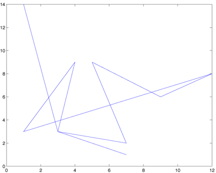
Notice that the line follows the path in order of the (x,y) coordinates. This is a bit messy, so we will want to change the plot output to plot as circles, rather than lines:
>> plot(x,y,'ko')
You can alter the appearance of the way Matlab graphics plot by
manipulating the third argument in the plot command. First, note that the
third argument is always surrounded by quotes. Next, there are two parts
to the third argument of the plot command-- the first is a plot color, the
second is a plot style. Characters such as `r' (red), `b' (blue), `g'
(green), may be used to alter the color of the plotted line or point.
Likewise, characters such as `.' (point plot), `+' (points are plotted as
crosses), `v' (points are plotted as upside-down triangles), '--' (plot as
dashed line), '-' (plot as solid line) may be used to alter the appearance
of the line. For example, if you would like to plot the $(x,y)$ pairs as a
red, dashed line, use 'r--' as the third argument of the plot command. You
may overlay plots by using the hold on command at the Matlab
prompt. This causes overlaying of graphics. For example, let's say that
you think that the above points obey some sort of relationship which is a
straight line. You know that the slope of the line is 3 and its
y-intercept is 2. In the equation:
>> a = 3;
>> b = 2;
>> ycalc = a.*x + b;
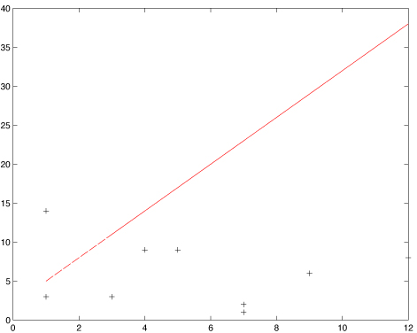
Therefore, we have two y vectors-- one that contains the actual data (y), and one that contains the calculated (or modeled if you prefer) relationship (ycalc). Let's plot the actual data as black crosses and the calculated relationship as a red dashed line:
>> plot(x,y,'k+')
>> hold on
>> plot(x, ycalc, 'r--')
This creates the following output:
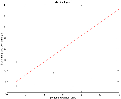
Now, you may wish to dress up your plot a little bit by adding a title and axes labels. Matlab will allow you to create a title using the title() command and make axis labels using the xlabel() ylabel() commands. So, let's add a title and axes labels to the figure:
>> title('My First Figure')
>> xlabel('Something without units')
>> ylabel('Something else with units (m)')
So, here is your finished figure:
Matlab is capable of graphing three variables as a contour plot. In this system, there are two independent variables which are varied along the x- and y-axes with a resultant z-value. The z-values may be contoured as long as the function at any point does not have multiple solutions.
In order to demonstrate how to make a contour plot in Matlab, we will use some built in Matlab functions to contour. For demonstration purposes, the function ``peaks'' is built into the Matlab system. In order to set a variable equal to this function, type:
>>Z = peaks;
This will fill the variable Z with the distribution and
return a 49x49 matrix of values representing the Z-values of
the distribution. If you wish to change the number of elements in
the matrix, simply put those numbers in the parentheses in the
``peaks'' function.
There are several ways to contour data. First, you can make a basic contour plot in which the contour lines represent a given interval. Second, you can contour using area contours which color the area in between contours a solid color. A third variation on the contour plot is to have uneven contour intervals. This is especially useful when contouring data which may have a wide range of Z-values which may be logarithmically distributed, for example. We will start with the simplest case of making a plain contour plot and build into the more complicated scenarios.
At this time, it is appropriate to introduce the concept of graphics
handles. Graphics handles are values that are returned when calling
some graphics functions which represent different aspects of the
graphic that you are working on. For example, if I called the
function >>contour(myDistribution), Matlab would return
several numbers which act as references to the graphic that I just
created with contour. These references are called
``handles'' and may be used to transfer the information created in
the graphics function to another function. For example, when contour
is called, handles are returned and may be put into the
clabel function which will label the appropriate contour
lines in the figure. An example of this is shown below.
To make a basic contour plot, we first need a distribution of data (a
matrix of Z-values). This may have been created from some data that
you have or we can call on Matlab's built in peaks function
to create a matrix of Z-values for demonstration purposes. First,
issue the command:
>>Z = peaks;
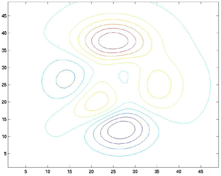
Next, you want to create a contour plot with ten contour lines and
keep the reference handles of the contour plot in the variables
c and h. To do this, issue the following command:
>>[c,h] = contour(Z,10);
Notice that the contour inverval of 10 is entered after the Z-value matrix. The result of this function is shown below:
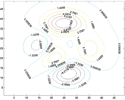
Now, let's put some labels on the contour lines. To do this, we will
use the clabel command. The clabel command takes
the contour plot's handles as arguments and will automatically label
the lines:
>>[c,h] = clabel(c,h);
The result of this operation is:
 % \includegraphics{Matlab1-6.ps}
title, xlabel, and ylabel
commands, you can add annotation to your contour plot.
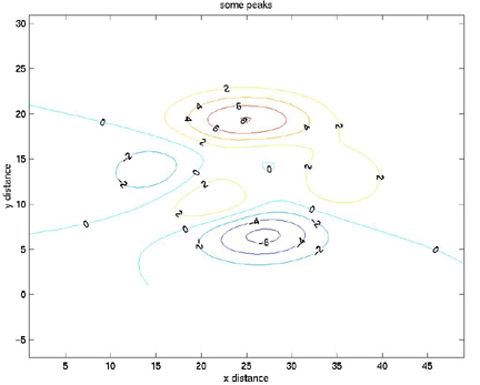
With contour, you can specify the size of each of the
elements of the Z-matrix by passing contour two additional
variables, a vector containing the X-values for each column in the
Z-matrix, and a vector containing the Y-values for each row in the
Z-matrix. For example, if the width of each of the elements in the
Z-matrix is one and the height of each element in the Z-matrix is
0.5, you can make two vectors which let contour know this
information. Use the incremental fill function (described above) to
set the values of the X- and Y- vectors to their appropriate values:
>>X=1:49;
>> Y = 1:.5:25;
>>[c,h] = contour(X,Y,Z,10);
>>clabel(c,h);
>>axis equal;
>> title('some peaks')
>> xlabel('x distance'), ylabel('y distance')
The axis equal command simply forces the size of the
X-increment to equal the size of the Y-increment on the axes of the
figure. If this is not done, Matlab will scale the axes to fit all of
the data onto the plot.
Here is the plot:
>>Z = peaks;
>>X=1:49;
>> Y = 1:.5:25;
mesh, surf, and surfl.>> mesh(X,Y,Z)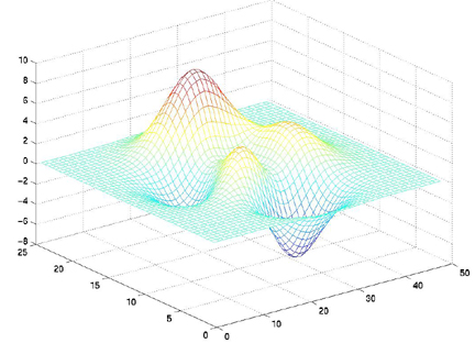
>> surf(X,Y,Z)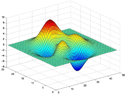
>> surfl(X,Y,Z)
>> shading interp
>> colormap pink
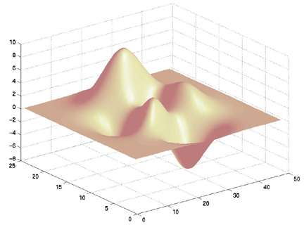
shading interp with that plot. The
shading function selects between faceted, flat, or interpolated shading.
Although it can take more graphics computations, the interpolated shading
usually looks best. We also used a colormap other than the default. The
colormap is a data structure that is ues to represent color values. It is
an array of three columns and some number of rows of RGB values. I have
made the same plot as above with a number of different built-in Matlab
colormaps:| colormap pink | colormap cool | colormap autumn | colormap winter | colormap flag | colormap copper |
|---|---|---|---|---|---|
|
|
|
|
|
|
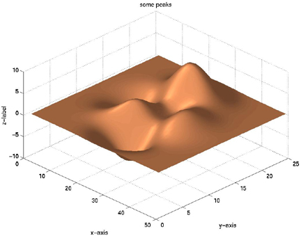
>> surfl(X,Y,Z)
>> shading interp
>> colormap copper
>> title('some peaks')
>> xlabel('x-axis'),ylabel('y-axis'),zlabel('z-label')
>> view(45,45)
| view(45,45) | view(270,90) | view(135,35) | |
|---|---|---|---|
 |
 |
 |
>>load E.txt, load N.txt, load H.txt>>plot(E,N,'k+')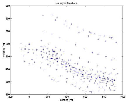
>> help griddata

 GRIDDATA Data gridding and surface fitting.
    ZI = GRIDDATA(X,Y,Z,XI,YI) fits a surface of the form Z = F(X,Y)
    to the data in the (usually) nonuniformly-spaced vectors (X,Y,Z)
    GRIDDATA interpolates this surface at the points specified by
    (XI,YI) to produce ZI.  The surface always goes through the data
    points.  XI and YI are usually a uniform grid (as produced by
    MESHGRID) and is where GRIDDATA gets its name.

    XI can be a row vector, in which case it specifies a matrix with
    constant columns. Similarly, YI can be a column vector and it
    specifies a matrix with constant rows.

    [XI,YI,ZI] = GRIDDATA(X,Y,Z,XI,YI) also returns the XI and YI
    formed this way (the results of [XI,YI] = MESHGRID(XI,YI)).

    [...] = GRIDDATA(...,'method') where 'method' is one of
        'linear'    - Triangle-based linear interpolation (default).
        'cubic'     - Triangle-based cubic interpolation.
        'nearest'   - Nearest neighbor interpolation.
        'v4'        - MATLAB 4 griddata method.
    defines the type of surface fit to the data. The 'cubic' and 'v4'
    methods produce smooth surfaces while 'linear' and 'nearest' have
    discontinuities in the first and zero-th derivative respectively.  All
    the methods except 'v4' are based on a Delaunay triangulation of the
    data.

    See also INTERP2, DELAUNAY, MESHGRID.
Basically, we need to tell griddata what the x and y grid looks like on
which it will operate. So I did this for our topography:
>> estep = (min(E)-max(E))/100

estep =

  -10.3468

>> estep = abs(estep)

estep =

   10.3468


>> e = [min(E):estep:max(E)]

>> nstep = (min(N)-max(N))/100

nstep =

   -6.0886

>> nstep = abs(nstep)

nstep =

    6.0886

>> n = [min(N):nstep:max(N)]
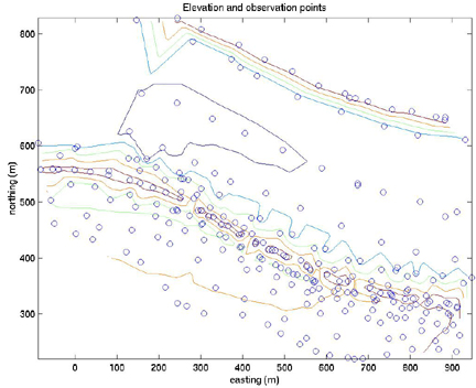
Those are the vectors of easting and northing positions for our grid.>> [xi,yi,zi] = griddata(E,N,H,e,n');
>> contour(xi,yi,zi)
>> hold on
>> plot(E,N,'o')
>> xlabel('easting (m)')
>> ylabel('northing (m)')
>> title('Elevation and observation points')
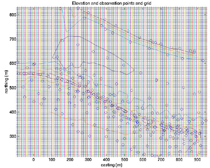
>> plot(xi,yi,'+')
>> title('Elevation and observation points and grid')
>> surfl(xi,yi,zi)
>> shading interp
>> colormap pink
>> hold on
>> plot3(E,N,H,'o')
>> title('oblique view of gridded data with observations plotted')
>> xlabel('easting(m)'),ylabel('northing(m)'),zlabel('Elevation(m)')
>> view (65,45)
