GLG410 programming in Matlab

The following lecture and demonstration of scripts and functions illustrate the real power of Matlab and the opportunity to get it to do some work for you. You can create these files in the text editor. They should be saved with a .m extension, and then run by typing their name (and adding arguements in the case of functions), but without the .m at the end.

Matlab scripts

One thing that you might ahve realized from your work in the last two weeks is that there can often be a lot of retyping of your work in order to account for some small changes. One powerful aspect of Matlab is the ability to write scriptswhich are essentially a series of Matlab commands strung together into a file the name of which is typed and the commands are executed in series.
here is a simple script that will say Hello:

%simple script to say hello world hello.m
fprintf('HELLO WORLD!\n');

and how I ran it and the outcome:

>> hello
HELLO WORLD!

See below for a bit more on the function fprintf. How about something more complicated with which you all might be familiar:
Here is a script that will load the topography data for today's assignment and then plot it and make a movie of it slowly rotating.

Have a look at the handout from Chapter 4 of Mastering Matlab 5.

Matlab functions

"When you use Matlab functions such as inv, abs, angle, and sqrt, matlab takes the variables that you pass it, computes the required results using your input, and then passes those results back to you. The commands evaluated by the function as well as any intermediate variables created by those commands are hidden. All you see is what goes in and what comes out (i.e., a function is a black box)."--p. 143 from Mastering Matlab 5.

Here is a simple function

function r = rads(degrees)
%this function takes an input angle in degrees and converts it to 
%radians
%JRA, 11.22.99

r = degrees * (pi/180);

Here is some Matlab action associated with it:

>> ls   

ans =

factor_of_safety.m
rads.m


>> help rads

 this function takes an input angle in degrees and converts it to 
 radians

>> rads(180)

ans =

    3.1416

Important points about the rads function:

Note that the first line always starts with the word function and the calling syntax and input and output variable.
The first set of contiguous comment lines (beginning with %) are the help text for the function.
Note that you have to be in the directory in which the function is or type its complete path or have the path to that directory added to your Matlab search path

Be sure to look at pages 144 and 145 for the rules for constructing a Matlab function.
Here are a couple of pretty useful commands that I have used in my functions:
fprintf is a Matlab function that can print a formatted text string to a file or the screen:

>> fprintf('here is a number = %.3f (that was the formatting)\n',2.5)
here is a number = 2.500 (that was the formatting)

The main points are that you put a formatted placeholder in the line (%.3f) which in this case says to format the number as a 3 decimal place floating point. The \n tells Matlab to start a new line. Note the newline and the formatting placeholder along with the text are in the quotes. Then the number follows and is placed where it should be. If you have more than one placeholder, Matlab puts the numbers in sequentially and you can actually evaluate an expression there:

>> fprintf('here is a number = %.3f (that was the formatting), and here is its half = %.\n',2.53f\n',2.5,2.5/2) 
here is a number = 2.500 (that was the formatting), and here is its half = 1.250

Factor of safety calculation by a function

In the world of engineering geology, a classic solution for the stability of a simple slope is called "infinite slope analysis." If we can calculate the driving and resisting stresses for a mass of material on a hillslope, the ratio of the sum of the resisting forces to the sum of the driving forces is called the factor of safety:
scheme

Where the variables are:
c' or c = cohesion of the material
rho rock is rock density
rho water is water density
theta is the dip angle of the failure surface
h is the vertical thickness of the slide mass
g is gravity
m is the fraction of saturated thickness such that m = 0 if the water table is just below the slide plane and m = 1 if the water table is at the ground surface.
phi is the angle of internal friction

FS > 1 => STABLE
FS < 1 => UNSTABLE
FS = 1 => CRITICAL

Here is a function that takes care of the calculation of the factor of safety for us.
Here is the help text:

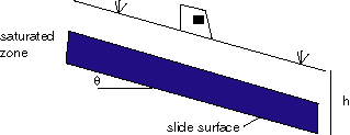
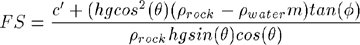
>> help factor_of_safety

 fs = factor_of_safety(c, h, theta, prock,m, phi)
 this function calculates the factor of safety for an infinite slope
 stability problem.
 See Arrowsmith notes
 note that suggested units are in parenthesis below
 JRA November 22,1999

 Variables:
        external
        c = cohesion (kg m^-1 s^-2)
        h = slide mass thickness (m)
        theta = slope angle in degrees
        prock = rock density (kg m^-3)
        m = fraction of saturated thickness (such that m = 0 if the water
                table is just below the slide surface and m = 1 if the
                water table is at the ground surface) (dimensionless)
        phi = angle of internal friction in degrees

        internal
        g = gravitational acceleration (m s^-2)
        pwater = water density (kg m^-3)
        driving = driving stresses
        resisting = resisting stresses

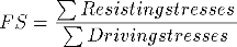
Here are some calculations to go with it:
This one is just past critical

>> factor_of_safety(11900,6,10,2000,1,8)
c = 11900.000, h = 6.000, theta = 10.000, prock = 2000.000, m = 1.000, phi = 8.000

ans =

    0.9896

Slope goes up, safety goes down:

>> factor_of_safety(11900,6,20,2000,1,8)
c = 11900.000, h = 6.000, theta = 20.000, prock = 2000.000, m = 1.000, phi = 8.000

ans =

    0.5076

Diminish saturation, safety goes up:

>> factor_of_safety(11900,6,10,2000,0.5,8)
c = 11900.000, h = 6.000, theta = 10.000, prock = 2000.000, m = 0.500, phi = 8.000

ans =

    1.1889

Increase internal friction, safety goes up

>> factor_of_safety(11900,6,10,2000,1,16)
c = 11900.000, h = 6.000, theta = 10.000, prock = 2000.000, m = 1.000, phi = 16.
000

ans =

    1.4042

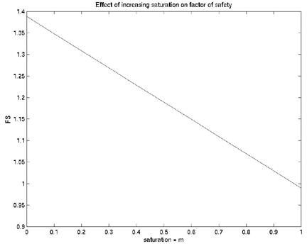
Now how about a few plots:

>> clear mm fss
>> for i=0:0.1:1                                    
fss = [fss factor_of_safety(11900,6,10,2000,i,8)];
mm = [mm i];                                      
end
Warning: Reference to uninitialized variable fss.
c = 11900.000, h = 6.000, theta = 10.000, prock = 2000.000, m = 0.000, phi = 8.000
Warning: Reference to uninitialized variable mm.
c = 11900.000, h = 6.000, theta = 10.000, prock = 2000.000, m = 0.100, phi = 8.000
c = 11900.000, h = 6.000, theta = 10.000, prock = 2000.000, m = 0.200, phi = 8.000
c = 11900.000, h = 6.000, theta = 10.000, prock = 2000.000, m = 0.300, phi = 8.000
c = 11900.000, h = 6.000, theta = 10.000, prock = 2000.000, m = 0.400, phi = 8.000
c = 11900.000, h = 6.000, theta = 10.000, prock = 2000.000, m = 0.500, phi = 8.000
c = 11900.000, h = 6.000, theta = 10.000, prock = 2000.000, m = 0.600, phi = 8.000
c = 11900.000, h = 6.000, theta = 10.000, prock = 2000.000, m = 0.700, phi = 8.000
c = 11900.000, h = 6.000, theta = 10.000, prock = 2000.000, m = 0.800, phi = 8.000
c = 11900.000, h = 6.000, theta = 10.000, prock = 2000.000, m = 0.900, phi = 8.000
c = 11900.000, h = 6.000, theta = 10.000, prock = 2000.000, m = 1.000, phi = 8.000
>> plot(mm,fss,'k')                                  
>> title('Effect of increasing saturation on factor of safety')
>> xlabel('saturation = m')
>> ylabel('FS')
>>

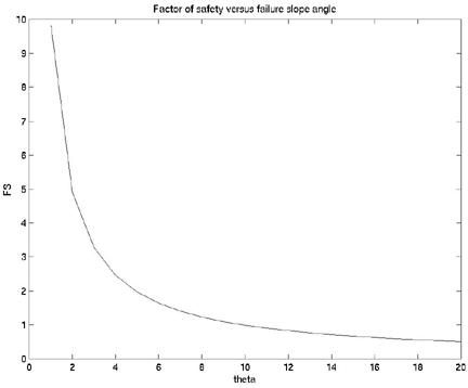
>> clear tt
>> clear fss
>> for i = 1:20                                        
fss = [fss factor_of_safety(11900,6,i,2000,1,8)];   
tt = [tt i];                                        
end                                                 
Warning: Reference to uninitialized variable fss.
c = 11900.000, h = 6.000, theta = 1.000, prock = 2000.000, m = 1.000, phi = 8.000
Warning: Reference to uninitialized variable tt.
c = 11900.000, h = 6.000, theta = 2.000, prock = 2000.000, m = 1.000, phi = 8.000
c = 11900.000, h = 6.000, theta = 3.000, prock = 2000.000, m = 1.000, phi = 8.000
c = 11900.000, h = 6.000, theta = 4.000, prock = 2000.000, m = 1.000, phi = 8.000
c = 11900.000, h = 6.000, theta = 5.000, prock = 2000.000, m = 1.000, phi = 8.000
c = 11900.000, h = 6.000, theta = 6.000, prock = 2000.000, m = 1.000, phi = 8.000
c = 11900.000, h = 6.000, theta = 7.000, prock = 2000.000, m = 1.000, phi = 8.000
c = 11900.000, h = 6.000, theta = 8.000, prock = 2000.000, m = 1.000, phi = 8.000
c = 11900.000, h = 6.000, theta = 9.000, prock = 2000.000, m = 1.000, phi = 8.000
c = 11900.000, h = 6.000, theta = 10.000, prock = 2000.000, m = 1.000, phi = 8.000
c = 11900.000, h = 6.000, theta = 11.000, prock = 2000.000, m = 1.000, phi = 8.000
c = 11900.000, h = 6.000, theta = 12.000, prock = 2000.000, m = 1.000, phi = 8.000
c = 11900.000, h = 6.000, theta = 13.000, prock = 2000.000, m = 1.000, phi = 8.000
c = 11900.000, h = 6.000, theta = 14.000, prock = 2000.000, m = 1.000, phi = 8.000
c = 11900.000, h = 6.000, theta = 15.000, prock = 2000.000, m = 1.000, phi = 8.000
c = 11900.000, h = 6.000, theta = 16.000, prock = 2000.000, m = 1.000, phi = 8.000
c = 11900.000, h = 6.000, theta = 17.000, prock = 2000.000, m = 1.000, phi = 8.000
c = 11900.000, h = 6.000, theta = 18.000, prock = 2000.000, m = 1.000, phi = 8.000
c = 11900.000, h = 6.000, theta = 19.000, prock = 2000.000, m = 1.000, phi = 8.000
c = 11900.000, h = 6.000, theta = 20.000, prock = 2000.000, m = 1.000, phi = 8.000
>> clf
>> plot(tt,fss,'k')
>> title('Factor of safety versus failure slope angle')
>> xlabel('theta')                                     
>> ylabel('FS')

Pages maintained by
Prof. Ramón Arrowsmith

Last modified November 23, 1999